How to freeze columns and rows in Google Sheets?

There are two ways you can freeze columns and rows in Google Sheets. By doing this, you can scroll through your table and still see your first columns or rows.

The Drag&Drop method

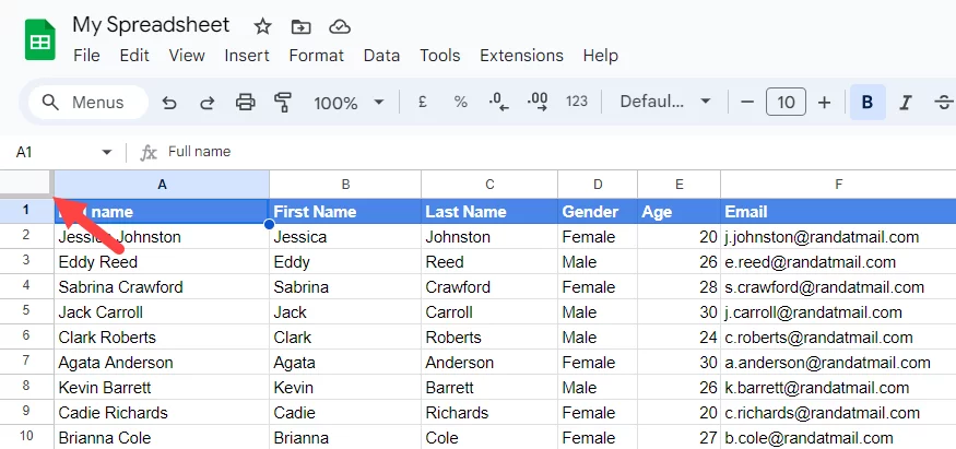
Find the empty square at the intersection of columns and rows. 

freeze-google-sheets-drag

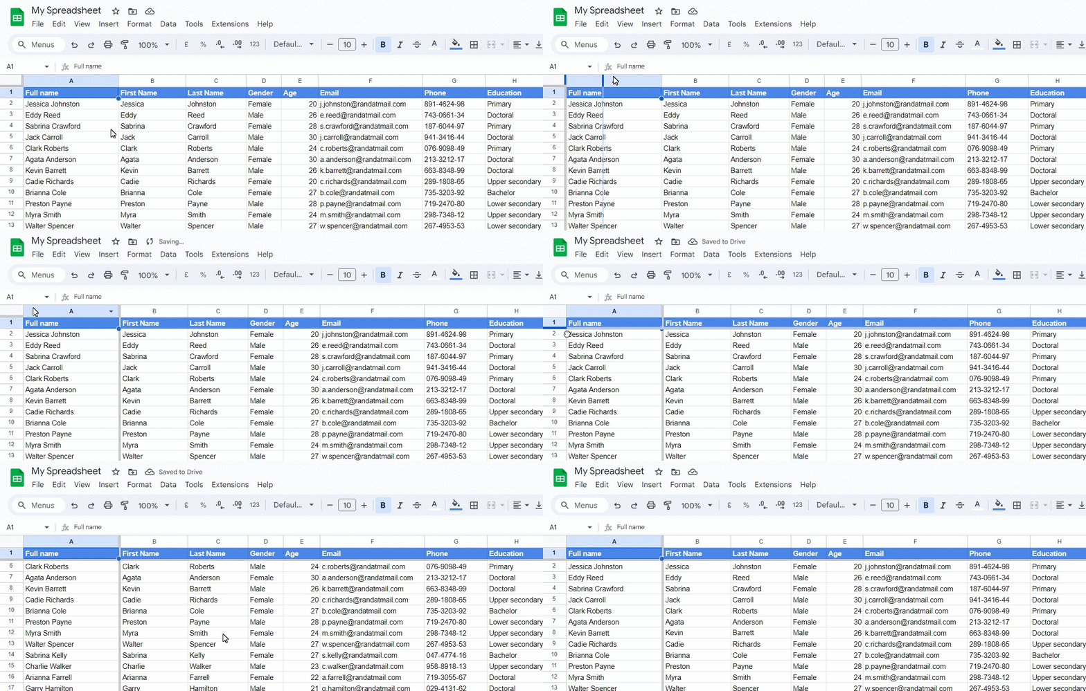
To freeze a row, drag its horizontal line down. To freeze a column, drag the vertical line to the right. Now, when you scroll down or to the right, the first row or column remains visible.

freeze-google-sheets-drag-drop

The Freeze function

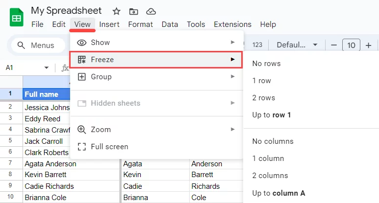
The second method is clicking View, Freeze, and selecting the rows or columns you want to freeze.

freeze-sheets

To undo the freezing of the column or rows, you can also drag it back to the initial position or click View, Freeze, and no rows or no columns.

Watch how to freeze columns and rows in Google Sheets

To see a video demo of all of Kanbanchi's features right here, please, accept functionality cookies.


More Google Workspace tips from Kanbanchi.

Also read: How to create a pivot table in Google Sheets?

Want to try the power of Kanbanchi and Google Workspace?

Start your free trial